| ||
Digital Collections of Real World ObjectsAppendix 1: BRDF FittingHendrik P.A. Lensch, Michael Goesele, and Hans-Peter Seidel |
Principle of BRDF FittingA lumitexel can be seen as a very sparsely sampled BRDF in a tabulated representation, typically with only four to ten entries. But instead of using the radiance samples captured in the lumitexel directly, we will represent the surface appearance by a mathematical BRDF model whose parameters have to be estimated with respect to the error between a lumitexel and the BRDF. This representation mainly has two advantages: Only the parameters of the BRDF model have to be stored instead of a list of radiance samples; and secondly, a BRDF model is defined even for incident and outgoing directions that have not been acquired, providing smooth data extrapolation. Many different parameterized BRDF models have been proposed (e.g. [Torrance and Sparrow, Larson]). Our method may be used with any parameterized BRDF model. We have chosen the computationally simple but general and physically plausible Lafortune model [Lafortune et al.] in its isotropic form with a single specular lobe:
This model uses only a handful of parameters: u and v are the local light and viewing directions. The diffuse color (i.e. the color in non-highlighted regions) is defined by the diffuse component As in the original work by Lafortune et al. [Lafortune et al.], we use the Levenberg-Marquardt method to fit the non-linear parameters of the model to the input data, minimizing the error between the lumitexel and the BRDF. Given an error measure between a single radiance sample and a given BRDF evaluated for the same viewing and lighting direction, the error of a whole lumitexel with respect to the BRDF can be defined as the mean of the errors of the individual radiance samples to the BRDF. The Levenberg-Marquardt optimization outputs not only the best-fit parameter vector, but also a covariance matrix of the parameters, which provides a rough idea of the parameters that could not be fitted well. We make use of this information in the following splitting and clustering algorithm. Clustering and BRDF GenerationUnfortunately, the number of radiance samples per lumitexels is too small to obtain faithful BRDF parameters from a single lumitexel. However, the parameters can be estimated accurately for a whole group or cluster of lumitexels, i.e. by increasing the number of samples. It must be ensured that the given lumitexels are partitioned into clusters so that each cluster corresponds to just one basic material of the object. Given a set of BRDFs, each lumitexel is associated with the BRDF, which minimizes the error between the measured radiance samples and the evaluated BRDF. Determining these clusters is a problem closely related to vector quantization [Gersho and Gray] and k-means clustering [Lloyd]. The general idea is to first fit a BRDF to an initial cluster consisting of all lumitexels. Then we generate two new BRDF models representing two new clusters. These BRDFs are generated by varying the parameters along the eigenvector of the covariance matrix with largest eigenvalue representing the direction of maximum variance in parameter space. The lumitexels from the original cluster are then distributed according to their distance to the generated BRDFs into the new clusters. New BRDF models are then fitted to the two clusters which best approximate the lumitexels in the new clusters. To obtain a clear separation between the generated clusters, we repeat the steps of distributing the lumitexels and BRDF fitting until the clusters are stable. We then recursively choose another cluster based on its current approximation error, split it, and redistribute the lumitexels and so on. This is repeated until the desired number of materials is reached.
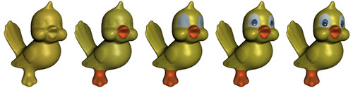
To accelerate our algorithm we determine the set of BRDFs and perform the clustering for an object only on a subset of all the acquired lumitexels. Once all clusters are found, the remaining lumitexels are distributed to the clusters and the BRDFs are refitted with the full data set. ProjectionAs can be seen in Figure 1A, the representation of an object by a collection of only a few clusters and corresponding BRDFs make the virtual object look artificial because real surfaces exhibit changes in the reflective properties even within a single material. These changes cannot be represented by a single BRDF per cluster since all lumitexels within the cluster would be assigned the same BRDF parameters. To obtain truly spatially varying BRDFs we must find a specific BRDF for each lumitexel. But the sparse input data does not allow fitting a reliable or even meaningful BRDF to a single lumitexel because each lumitexel consists of only a few radiance samples. The solution is to project each lumitexel into a basis of BRDFs, i.e. to represent the BRDF
with t1, t2, ..., tm, being scalar weights. This forces the space of solutions (i.e. the possible BRDFs for a pixel) to be plausible since the basis BRDFs are already reliably fitted to a large number of radiance samples. Given this basis of BRDFs, the weights for a lumitexel can be found by a least square optimization. Compared to the non-linear fitting of BRDF model parameters (see the Section "Principle of BRDF Fitting" above), we now have a linear problem to solve with a smaller degree of freedom and even more constraints. A stable and meaningful solution can therefore be found although only a few samples are available per lumitexel. References[Gersho and Gray] A. Gersho and R. Gray. Vector Quantization and Signal Compression. Kluwer Acad. Publishers, 1992. [Lafortune et al.] E. Lafortune, S. Foo, K. Torrance, and D. Greenberg. Non-Linear Approximation of Reflectance Functions. In Proc. SIGGRAPH, pages 117-126, August 1997. [Larson] G. Ward Larson. Measuring and Modeling Anisotropic Reflection. In Proc. SIGGRAPH, pages 265-272, July 1992. [Lloyd] S. Lloyd. Least squares quantization in PCM. IEEE Trans. on Information Theory, IT-28:129-137, 1982. [Torrance and Sparrow] K. Torrance and E. Sparrow. Theory for Off-Specular Reflection from Roughened Surfaces. Journal of Optical Society of America, 57(9), 1967. Copyright© 2002 Hendrik P.A. Lensch, Michael Goesele, and Hans-Peter Seidel. | |